Raw Data Checks
Channel Intensity Profiles (CIP)
Average intensity is plotted for each slice (in the order: Phase, Z, Angle, Time) where each channel is assigned an arbitrary color: 1st channel = red, 2nd = green, 3rd = blue, subsequent = black. This helps judge bleaching and whether all angles show a similar intensity (as they should).
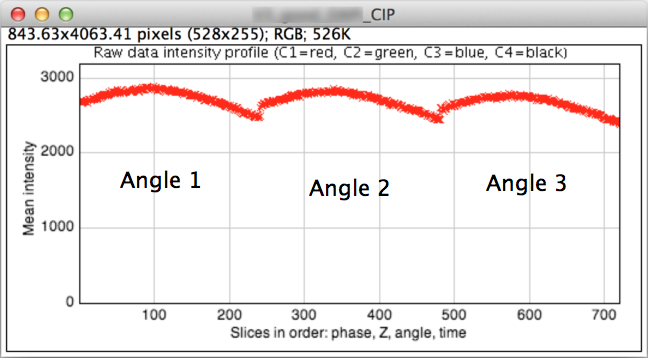
Figure 2a. Intensity profile for single-channel image without bleaching.
An overall summary statistic is reported for each channel: total intensity variation (%). This is for a 9-Z window about the central Z-slice. The following additional statistics each contribute to the total intensity variation, enabling the source of the problem to be identified:
estimated intensity decay (%), due to photobleaching
maximum intensity difference between angles (%), due to miscalibration
relative intensity fluctuations (%), due to illumination flicker
Examples of each of each of these problems are shown in Figures 2b, 2c and 2d below, respectively. Note that typically around 50% total intensity variation can be tolerated, depending on the minimum signal-to-noise level (since this impacts modulation contrast to noise).
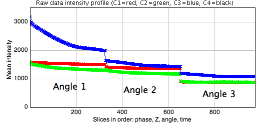
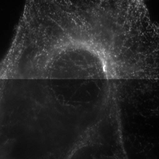
Figure 2b. Left: Intensity profile for 3-channel image showing significant bleaching in the third channel (blue). Right: a Z-slice from this image split to show angle 1 (top) and angle 3 (bottom), illustrates that bleaching occurs during acquisition of angles 1 and 2.
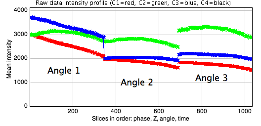
Figure 2c. Intensity profile for a 3-channel image showing systematic intensity differences between the slices of the 3 angles.
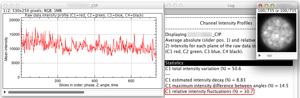
Figure 2d. Intensity profile for a 1-channel image showing a significant slice-to-slice intensity fluctuations (due to unstable illumination).
Motion & Illumination Variation (MIV)
This check highlights features that change in-between recording data for different angles. Each angle (assumes 3!) is assigned a color: Cyan, Magenta, or Yellow, meaning that if a feature is present in all angles it will appear C+M+Y=White, or will exhibit the color of a specific angle(s) if not (the color scheme chosen here is intended to make the distinction between angles and channels clear). The reconstruction algorithm assumes that all features are sampled at each angle, and features that move or experience different illumination intensity for different angles (or phases) will result in artifacts.
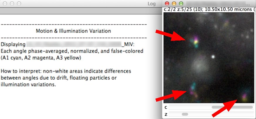
Figure 2e. False-colored ‘MIV’ check image, where white regions have intensities in the same proportion across all angles. The sample contained non-fixed features that moved in-between data acquisition for the different angles: these can be seen as colored spots (highlighted in this figure with red arrows).
Fourier Projections (FPJ)
This check is not turned on by default in the main dialog, since it it requires a sample that fills a large porportion of the field of view and is mainly intended for diagnosis of hardware issues.
2D Fourier Transforms of the raw data are taken, and projected over all phases and angles. To make best use of the available display range, i.e. to enhance the contrast of the relevant features in this projection, the “bright” central region containing the offset and low frequencies is masked out. Furthermore, a logarithmic display scale of log(Amplitude^2) is used. There are sliders for channel and time if present.
Where features in the raw data are in-focus and their intensities are modulated by the illumination pattern, 2D FFTs of each plane in the raw SI data should show 1st and 2nd order spots along a line perpendicular to the angle of illumination pattern stripes. Blurred, missing or extra spots may indicate problems with the illumination pattern (although sparse samples may lack clear spots in the FFT). Note that images with XY sizes that are not a power of 2 (256x256, 512x512 and so on are power of 2) require padding, which may lead to inferior results.
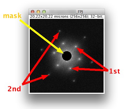
Figure 2f. Projection of 2D Fourier transforms for a good SIM dataset that fills the field of view. Here the first and second order spots (marked in red) are clearly visible and clean/sharp. Note that the plot is symmetrical about the centre, with low frequencies in the middle and high frequencies at the edges. The central mask blanking out the bright zero order / offset peak and low frequencies is marked with a yellow arrow.
Modulation Contrast (MCN)
The Modulation Contrast-to-Noise Ratio (MCNR) is a ratio of SI illumination pattern strength to noise strength - values less than 3 are inadequate (purple), values ~6 are adequate (red), values of ~12 are good (orange), values of ~18 are very good (yellow) and values of ~24 or better are excellent (white). NB. the display range must not be changed from 0 to 24 for meaningful interpretation of the Look-Up Table. The check reports an average MCNR value for auto-thresholded image features (Otsu method), and an estimate for the optimal Wiener filter parameter for OMX data reconstruction based on this.
If the illumination pattern at a given feature is overpowered by the noise, reconstruction will fail - any super-resolution features observed in such regions cannot be trusted. Note that contrast is key, and even high signal intensities may be inadequate where contrast is poor.
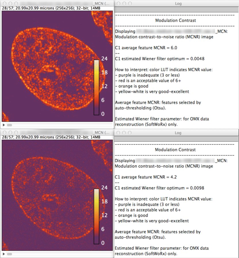
Figure 2g. Modulation Contrast-to-Noise (MCN) images for a pair of raw SIM datasets acquired at medium and low signal-to-noise ratios (top and bottom, respectively). The bottom image has inadequate MCN to give a good, high resolution reconstruction.